Down to the Bottom – Weights Update When Minimizing the Error of the Cost Function for Linear Regression

The cost function for Linear Regression is Mean Squared Errors. It goes like below:

J(\theta) = \frac{1}{m}\sum_{i=1}^{m}\left ( \hat{y}^{(i)}-y^{(i)} \right )^{2} = \frac{1}{m}\sum_{i=1}^{m}\left( h_{\theta}\left ( x^{(i)}\right ) -y^{(i)} \right )^{2}

x^{i} is the data point i in the training dataset. h_{\theta}\left ( x^{(i)}\right ) is a linear function for the weights and the data input, which is

h_{\theta}(x)=\theta^{T}x = \theta_{0}x_{0}+ \theta_{1}x_{1}+\theta_{2}x_{2}+\theta_{3}x_{3}+\cdot\cdot\cdot+\theta_{j}x_{j}

To find the best weights that minimize the error, we use Gradient Descent to update the weights. If you have been following Machine Learning courses, e.g. Machine Learning Course on Coursera by Andrew Ng, you should have learned that to update the weights, you need to repeat the process below until it converges:

\theta_{j} = \theta_{j} - \alpha\frac{1}{m}\sum_{i=1}^m(h_{\theta}(x^{(i)})-\hat{y})\cdot x_j^{(i)} for j=0…n (n features)

In Andrew Ng’s course, it it also expanded to:
\theta_{0} = \theta_{0} - \alpha\frac{1}{m}\sum_{i=1}^m(h_{\theta}(x^{(i)})-\hat{y})\cdot x_0^{(i)}
\theta_{1} = \theta_{1} - \alpha\frac{1}{m}\sum_{i=1}^m(h_{\theta}(x^{(i)})-\hat{y})\cdot x_1^{(i)}
\theta_{2} = \theta_{2} - \alpha\frac{1}{m}\sum_{i=1}^m(h_{\theta}(x^{(i)})-\hat{y})\cdot x_2^{(i)}

\theta_{j} = \theta_{j} - \alpha\frac{1}{m}\sum_{i=1}^m(h_{\theta}(x^{(i)})-\hat{y})\cdot x_j^{(i)}

However, when I first studied the course a couple of years ago, I did get stuck for a little trying to figure out where that exactly came from. I wish someone had given me some more concrete expansion so I could figure it out faster. Let me do that here so you can examine the detailed breakdown and get through this stage quickly. That’s the whole objective of this blog.

Let’s make this less abstract by putting down exact data point with a small sample and feature sizes. Let’s say, we have a set of data with 4 features like below and we only select 3 samples from it for simplicity.
\begin{bmatrix} x_0^{(1)} & x_1^{(1)}  & x_2^{(1)}  & x_3^{(1)}  & x_4^{(1)}  \\ x_0^{(2)} & x_1^{(2)}  & x_2^{(2)}  & x_3^{(2)}  & x_4^{(2)} \\ x_0^{(3)} & x_1^{(3)}  & x_2^{(3)}  & x_3^{(3)}  & x_4^{(3)} \\ x_0^{(4)} & x_1^{(4)}  & x_2^{(4)}  & x_3^{(4)}  & x_4^{(4)} \\ x_0^{(5)} & x_1^{(5)}  & x_2^{(5)}  & x_3^{(5)}  & x_4^{(5)}  \end{bmatrix} \cdot\begin{bmatrix}\theta_0 \\ \theta_1 \\ \theta_2 \\ \theta_3\\ \theta_4  \end{bmatrix}

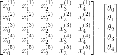
The prediction for each sample is:

\hat{y}^{(1)} = \theta_{0}x_{0}^{(1)}+ \theta_{1}x_{1}^{(1)}+\theta_{2}x_{2}^{(1)}+\theta_{3}x_{3}^{(1)}+\theta_{4}x_{4}^{(1)}
\hat{y}^{(2)} = \theta_{0}x_{0}^{(2)}+ \theta_{1}x_{1}^{(2)}+\theta_{2}x_{2}^{(2)}+\theta_{3}x_{3}^{(2)}+\theta_{4}x_{4}^{(2)}
\hat{y}^{(3)} = \theta_{0}x_{0}^{(3)}+ \theta_{1}x_{1}^{(3)}+\theta_{2}x_{2}^{(3)}+\theta_{3}x_{3}^{(3)}+\theta_{4}x_{4}^{(3)}

In this case the cost function wold be:

J(\theta) = \frac{1}{m}\sum_{i=1}^{m}\left ( \hat{y}^{(i)}-y^{(i)} \right )^{2} = \frac{1}{m}\sum_{i=1}^{m}\left( h_{\theta}\left ( x^{(i)}\right ) -y^{(i)} \right )^{2}
=((\theta_{0}x_{0}^{(1)}+ \theta_{1}x_{1}^{(1)}+\theta_{2}x_{2}^{(1)}+\theta_{3}x_{3}^{(1)}+\theta_{4}x_{4}^{(1)})-y^{1})^2 +((\theta_{0}x_{0}^{(2)}+ \theta_{1}x_{1}^{(2)}+\theta_{2}x_{2}^{(2)}+\theta_{3}x_{3}^{(2)}+\theta_{4}x_{4}^{(2)})-y^{2}))^2 +((\theta_{0}x_{0}^{(3)}+ \theta_{1}x_{1}^{(3)}+\theta_{2}x_{2}^{(3)}+\theta_{3}x_{3}^{(3)}+\theta_{4}x_{4}^{(3)})-y^{3}))^2

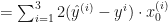
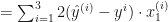
To minimize the cost, we need to find the partial derivatives of each \theta . The method to update the weights is

\theta_j = \theta_j - \alpha\frac{\partial}{\partial\theta_j}J(\theta)

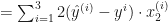
Let’s find the derivative of the \theta s here, step by step. From the cost function above, by applying Chain Rule, we have:
\frac{\partial}{\partial\theta_0} J(\theta) =
2((\theta_{0}x_{0}^{(1)}+ \theta_{1}x_{1}^{(1)}+\theta_{2}x_{2}^{(1)}+\theta_{3}x_{3}^{(1)}+\theta_{4}x_{4}^{(1)}) - y^1 )\cdot x_{0}^{(1)}
+ 2((\theta_{0}x_{0}^{(2)}+ \theta_{1}x_{1}^{(2)}+\theta_{2}x_{2}^{(2)}+\theta_{3}x_{3}^{(2)}+\theta_{4}x_{4}^{(2)})-y^2 )\cdot x_{0}^{(2)}
+ 2((\theta_{0}x_{0}^{(3)}+ \theta_{1}x_{1}^{(3)}+\theta_{2}x_{2}^{(3)}+\theta_{3}x_{3}^{(3)}+\theta_{4}x_{4}^{(3)})-y^3 )\cdot x_{0}^{(3)}
= \sum_{i=1}^3 2(\hat{y}^{(i)}-y^i)\cdot x_0^{(i)}

Do the same for the rest of the \theta s

\theta_1:
\frac{\partial}{\partial\theta_1} J(\theta) =
2((\theta_{0}x_{0}^{(1)}+ \theta_{1}x_{1}^{(1)}+\theta_{2}x_{2}^{(1)}+\theta_{3}x_{3}^{(1)}+\theta_{4}x_{4}^{(1)}) - y^1 )\cdot x_{1}^{(1)}
+ 2((\theta_{0}x_{0}^{(2)}+ \theta_{1}x_{1}^{(2)}+\theta_{2}x_{2}^{(2)}+\theta_{3}x_{3}^{(2)}+\theta_{4}x_{4}^{(2)})-y^2 )\cdot x_{1}^{(2)}
+ 2((\theta_{0}x_{0}^{(3)}+ \theta_{1}x_{1}^{(3)}+\theta_{2}x_{2}^{(3)}+\theta_{3}x_{3}^{(3)}+\theta_{4}x_{4}^{(3)})-y^3 )\cdot x_{1}^{(3)}
= \sum_{i=1}^3 2(\hat{y}^{(i)}-y^i)\cdot x_1^{(i)}

\theta_2:
\frac{\partial}{\partial\theta_2} J(\theta) =
2((\theta_{0}x_{0}^{(1)}+ \theta_{1}x_{1}^{(1)}+\theta_{2}x_{2}^{(1)}+\theta_{3}x_{3}^{(1)}+\theta_{4}x_{4}^{(1)}) - y^1 )\cdot x_{2}^{(1)}
+ 2((\theta_{0}x_{0}^{(2)}+ \theta_{1}x_{1}^{(2)}+\theta_{2}x_{2}^{(2)}+\theta_{3}x_{3}^{(2)}+\theta_{4}x_{4}^{(2)})-y^2 )\cdot x_{2}^{(2)}
+ 2((\theta_{0}x_{0}^{(3)}+ \theta_{1}x_{1}^{(3)}+\theta_{2}x_{2}^{(3)}+\theta_{3}x_{3}^{(3)}+\theta_{4}x_{4}^{(3)})-y^3 )\cdot x_{2}^{(3)}
= \sum_{i=1}^3 2(\hat{y}^{(i)}-y^i)\cdot x_2^{(i)}

\theta_3:
\frac{\partial}{\partial\theta_3} J(\theta) =
2((\theta_{0}x_{0}^{(1)}+ \theta_{1}x_{1}^{(1)}+\theta_{2}x_{2}^{(1)}+\theta_{3}x_{3}^{(1)}+\theta_{4}x_{4}^{(1)}) - y^1 )\cdot x_{3}^{(1)}
+ 2((\theta_{0}x_{0}^{(2)}+ \theta_{1}x_{1}^{(2)}+\theta_{2}x_{2}^{(2)}+\theta_{3}x_{3}^{(2)}+\theta_{4}x_{4}^{(2)})-y^2 )\cdot x_{3}^{(2)}
+ 2((\theta_{0}x_{0}^{(3)}+ \theta_{1}x_{1}^{(3)}+\theta_{2}x_{2}^{(3)}+\theta_{3}x_{3}^{(3)}+\theta_{4}x_{4}^{(3)})-y^3 )\cdot x_{3}^{(3)}
= \sum_{i=1}^3 2(\hat{y}^{(i)}-y^i)\cdot x_3^{(i)}

\theta_4:
\frac{\partial}{\partial\theta_4} J(\theta) =
2((\theta_{0}x_{0}^{(1)}+ \theta_{1}x_{1}^{(1)}+\theta_{2}x_{2}^{(1)}+\theta_{3}x_{3}^{(1)}+\theta_{4}x_{4}^{(1)}) - y^1 )\cdot x_{4}^{(1)}
+ 2((\theta_{0}x_{0}^{(2)}+ \theta_{1}x_{1}^{(2)}+\theta_{2}x_{2}^{(2)}+\theta_{3}x_{3}^{(2)}+\theta_{4}x_{4}^{(2)})-y^2 )\cdot x_{4}^{(2)}
+ 2((\theta_{0}x_{0}^{(3)}+ \theta_{1}x_{1}^{(3)}+\theta_{2}x_{2}^{(3)}+\theta_{3}x_{3}^{(3)}+\theta_{4}x_{4}^{(3)})-y^3 )\cdot x_{4}^{(3)}
= \sum_{i=1}^3 2(\hat{y}^{(i)}-y^i)\cdot x_4^{(i)}

If you are at first unclear about the functions and notations in the courses or some other documentations, I hope the expansion above would help you figure it out.

Leave a comment