Video Classification using CNN+ RNN


This article explores how to perform video classification using CNN+RNN models. The use case here is to have a system to monitor the driver on the car, and check if the driver is drowsy or not. The complete system would include a device with camera that hosts the built model that can be installed on a car. The hardware deployment part is out of the scope of this article. If you are interested in it, feel free to put in comments. I’ll share the link to my code there. The focus of this article is video classification model building and comparison.

The nature of videos is a sequence a consecutive frames. When it comes to video classification or event recognition, it is often necessary to process multiple frames together to make sense of what is happening. This article use an approach that combines the image feature extraction of convolutions and temporal information processing of RNN. There can be different approaches. Initially, I started with ConvLSTM (Convolutional Long Short-Term Memory). However, I realised that the overall accuracy is low initially and it overfits. While I tried different methods to optimise the same model, I also explored further and tried LRCN (Long-term Recurrent Convolutional Network). LRCN produced better stability and there is much less sign of overfitting. It also trains faster. I’ll give an overview of both approaches before sharing the step-by-step code.

Approach 1: ConvLSTM (Convolutional Long Short-Term Memory)

This is an existing Keras class (ConvLSTM2D layer, n.d.) that can be used. The structure of ConvLSTM network is essentially the same as a typical LSTM. The difference is that inside each cell, the matrix multiplication between input and weights in the input, forget and output gates is changed to convolutions. This way, it can take image inputs directly, extracting the features inside the LSTM cells and feeding them to the next time step to be combined with the convolution result of the next input frame. There is a research paper that provided a good grasp of the concept and technical details (Medel, 2016).

The diagram below was drawn based on my understanding of the ConvLSTM model and our implementation in this project.

ConvLSTM model

Approach 2: LRCN (Long-term Recurrent Convolutional Network)

Compared to the ConvLSTM approach, it requires the image to be processed first before feeding into the LSTM cell. Compared to ConvLSTM, it does perform less rounds of convolution computation as what is fed into the input of LSTM is the flattened vector output from the earlier convolutional layers. The diagram below illustrates the architecture of the model.

LRCN Model

One key difference between ConvLSTM and LRCN in input is that the inputs (x0, x1, x2…xt) in ConvLSTM are picture data directly while the input in LRCN are vectors as the result of CNN layers.


Data Acquisition and Preprocessing

To start with, we need to get the data needed for training. Fortunately enough, there is a good labelled dataset from National Tsing Hua University (Ching-Hua Weng, 2016). They were very kind and shared the data generously.

Dataset Info

Each video is about 100 seconds long and there is a mixture of drowsy sections and alert sections. For example, one of the videos has the following frames:

Frame-wise Labelling

As you can see that each video has frames of different classes. For model training, you need videos of the same type to the model for training. Therefore, the dataset cannot be used as-is. Therefore, I decided to make video clips of the same label (all “0” frames or “1” frames). The design is to build 10-second videos clips of the same type out of the given dataset. The assumption (human judgement) here is that a 10-second video is long enough to give good information to determine whether the driver is drowsy or not, while it is short enough to be processed with limited compute power.

Therefore, the training and testing data was produced by processing the videos obtained and made into 10-second clips. To do this, I developed a function based on OpenCV to read 10 seconds of frames (10s * 30 fps=300 frames) of the same label and save as a video file. Frame by frame, the corresponding label in the txt file is checked before it is saved. This makes sure the video clip is of the same type (drowsy or non-drowsy).

# Import opencv
import cv2
# Import operating sys
import os
# Import matplotlib
from matplotlib import pyplot as plt# Using batch to track videos
batch = 26# Establish capture object
cap = cv2.VideoCapture(os.path.join('data','sleepyCombination.avi'))

# Properties that can be useful later.
height = int(cap.get(cv2.CAP_PROP_FRAME_HEIGHT))
width = int(cap.get(cv2.CAP_PROP_FRAME_WIDTH))
fps = cap.get(cv2.CAP_PROP_FPS)
total_frames = cap.get(cv2.CAP_PROP_FRAME_COUNT)

#The length of each clip in seconds
num_sec = 10
# 1 for drowsy, 0 for alert.
capture_value = str(1)

# Open the Text File for tagging
with open(os.path.join('data','009_sleepyCombination_drowsiness.txt')) as f:
content = f.read()

# Helper counters.
# i tracking how many frames have been saved into clips
# j tracking where the current frame is.
i=0
j=0

# To make sure the number of labels is exactly the same as the number of frames before proceeding.
print(len(content))
print(total_frames)# Video Writer
# If there are still enough frames to be processed. Making the 1st video clip.
if j< total_frames - num_sec*fps:
video_writer = cv2.VideoWriter(os.path.join('data','class'+capture_value,'class'+capture_value + '_batch_'+str(batch)+'_video'+'1.avi'), cv2.VideoWriter_fourcc('P','I','M','1'), fps, (width, height))
# Loop through each frame
for frame_idx in range(int(cap.get(cv2.CAP_PROP_FRAME_COUNT))):
# Read frame
ret, frame = cap.read()
j+=1
# Show image
#cv2.imshow('Video Player', frame)

if ret==True:
if content[frame_idx] == capture_value:
# Write out frame
video_writer.write(frame)
i+=1
if i > num_sec*fps:
break
# Breaking out of the loop
if cv2.waitKey(10) & 0xFF == ord('q'):
break

# Release video writer
video_writer.release()# Making the 2nd clip
if j< total_frames - num_sec*fps:
video_writer = cv2.VideoWriter(os.path.join('data','class'+capture_value,'class'+capture_value+ '_batch_'+str(batch)+'_video'+'2.avi'), cv2.VideoWriter_fourcc('P','I','M','1'), fps, (width, height))
for frame_idx in range(i+1, int(cap.get(cv2.CAP_PROP_FRAME_COUNT))):
ret, frame = cap.read()
j+=1
#cv2.imshow('Video Player', frame)
if ret==True:
if content[frame_idx] == capture_value:
video_writer.write(frame)
i+=1
if i > 2*num_sec*fps:
break

# Release video writer
video_writer.release()

# Making the 3rd clip
if j< total_frames - num_sec*fps:
video_writer = cv2.VideoWriter(os.path.join('data','class'+capture_value,'class'+capture_value+ '_batch_'+str(batch)+'_video'+'3.avi'), cv2.VideoWriter_fourcc('P','I','M','1'), fps, (width, height))
for frame_idx in range(i+1, int(cap.get(cv2.CAP_PROP_FRAME_COUNT))):
ret, frame = cap.read()
j+=1
#cv2.imshow('Video Player', frame)
if ret==True:
if content[frame_idx] == capture_value:
video_writer.write(frame)
i+=1
if i > 3*num_sec*fps:
break
# Release video writer
video_writer.release()

### Continue making 4th, 5th..in the same way. Based on the data given,
### each video can be made into 8-9 clips.

# Close down everything at the end.
cap.release()
cv2.destroyAllWindows()

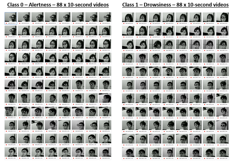
After preparation, we have the following set of videos for training and testing:

Video Clips Prepared

One thing important to mention here is about frame sampling. On a video that is 30 frames per second, if you take 20 consecutive frames, for example, it is less than 1 second of content. It does not contain sufficient information for inference. Each frame should look similar as well because in a car-driving setting, the changes are not drastic. Therefore, you can consider to do some down sampling. What I did was to take the 20 frames out of 200 frames, skipping 10 frames at each step, this captures 6–7 seconds of information and good enough to determine if the driver is drowsy or not. One key consideration of the design is also about the eventual deployment of the target solution. If we were to deploy the model on an edge device, what is a good number of frames that can be processed as one sequence. Based on the experiments with sample videos, 20 frames as one sequence is a good balance between sufficient information and the limited compute power. Just think about the nature of the type of videos we need to eventually. It is camera captures of drivers. This type of videos usually does not have drastic changes across frames. When a driver becomes drowsy, it is also a gradual change process. So, it is not critical to capture very single frame.


Model Building

The detailed model building code and explanation can be found in my other blog: https://medium.com/@junfeng142857/real-time-video-classification-using-cnn-rnn-5a4d3fe2b955

Iterations and findings

In the initial model, I tried feeding the entire 10-second video (300) frames into the model. This turned out too big for the compute power available to us. The biggest computer we are using is the one provided by Google Colab pro+ subscription which provides:

  • RAM: 90GB
  • GPU: NVIDIA-SMI 460.32.03; Driver Version: 460.32.03; CUDA Version: 11.2; GPU Memory size: 40GB

Even with the compute power above, the model was not able to train as it crashes the machine. Therefore, I decided to reduce the number of frames per sequence. This consideration is not just for training. We also need to consider eventual deployment which is on an edge device that has much less compute power. To decide what number of frames is good, I took the following factors into consideration:

  1. Deploy-ability. After quick deployment test on Raspberry Pi, a TensorFlow model with 20 frames per sequence can run at near full CPU. 40 frames and above had the risk of device failure.
  2. Model performance. I also compared how the number of frames per sequence impacts the model stability and accuracy, and noticed that 20 frames yields better accuracy than 40 frames across both approaches!

On top of the above, 20 frames per second also has a higher training speed. Therefore, it is good to keep the model at 20 frames per second.

In addition, through running iterations of training with both models, it was noticed that ConvLSTM has overall better accuracy at 20 frames per sequence, but LRCN has clear advantages.

  1. ConvLSTM has better test accuracy. In V1-40-frame, LRCN has a higher accuracy than ConvLSTM (ConvLSTM 70% vs LRCN 84%). In V2-20-frame training, LRCN has a lower accuracy (ConvLSTM 93% vs LRCN 84%). This shows that LRCN is more stable and ConvLSTM’s accuracy varies based on data. This difference can come from the complexity of the ConvLSTM model. Convolution is done at the input, forget and output gates. So longer sequence may give the model too much information to process so that it negatively impacted the performance.
  2. ConvLSTM also has higher tendency to overfit. Based on the training history, ConvLSTM has a higher tendency of overfitting. This should also be from the model complexity of ConvLSTM.
  3. LRCN has a higher training and inference speed. For a batch_size of 4, LRCN trains at 52 ms/step while ConvLSTM is at 884 ms/step.

To optimise the model, to following were also done during the training process.

  1. When preparing data, the data between the classes were balanced. There are the same number of videos in the dataset for each class.
  2. Dropout layers were added to the models. This helped reduce overfit.

Reference:

Video tutorials and documentations referenced:

Dataset:

Ching-Hua Weng, Ying-Hsiu Lai, Shang-Hong Lai, Driver Drowsiness Detection via a Hierarchical Temporal Deep Belief Network, In Asian Conference on Computer Vision Workshop on Driver Drowsiness Detection from Video, Taipei, Taiwan, Nov. 2016

Literature Mentioned:

  • Medel, J. R. (2016). Anomaly Detection Using Predictive Convolutional Long Short Term Memory Units . Rochester Institute of Technology.

IoT LoRaWAN Payload Decoding

IoT devices typically transmit data over a long distance with limited power available. LoRaWAN protocol is design for this purpose. It also brings other advantages such as

  • Scalability: LoRaWAN networks can support millions of devices, making it suitable for wide-scale deployments.
  • Security: LoRaWAN has built-in encryption and security at the network and application layers. This ensures that data transmitted between devices and the network server is secure.

Recently, I’ve had some fun playing with some IoT devices and looking closely into how the payload can be encoded and decoded. This article is meant to focus on the payload decoding. However, it is good to give an overview the setup as background information.

The system setup consists of the following main components.

  1. Weather station set up to collect 8 metrics.
  2. Helium Network setup for collection raw data
  3. Data Parsing and Machine Learning Model Building on Colab
  4. Model Deployment on www.pythonanywhere.com

Data is collected through 8-in-1 weather station. Purchased from Seeed Studio.

It collects the following metrics:

Data is transmitted through Helium Network and collected into Google Sheet.

This is an example of debug payload on the Helium console:

The payload is base64 encoded. For example, the string AQEwQAAAJVYAAAg= when decoded into Hex it is:

01 01 30 40 00 00 25 56 00 00 08

It carries the actual weather data we are collecting such as temperature, humidity, wind speed etc. The encoding logic is defined by the product provider, and is shared in JavaScript code: S2120-Helium decoder. In my project, I need to convert the JavaScript code into Python for Machine Learning model building. That process allowed me to understand the logic in-depth.

Data is interpreted in the following structure:

The dataId at the beginning determines the type of data the subsequent numbers encode.

If dataId=01, the subsequent numbers encode Temperature, Humidity, Light Intensity, UV Index, and Wind Speed.

If dataId=02, the subsequent numbers encode Wind Direction, Rain Gauge, and Barometric Pressure.

The tables below illustrate how the numbers are decoded layer by layer following the logic.

General Regression Neural Network (GRNN) Illustrated in Excel

Unlike other popular Machine Learning algorithms, there is not as much content on the Internet for beginners on General Regression Neural Network (GRNN). Wikipedia: https://lnkd.in/g2zktChp

I’ve built an Excel workbook to illustrate the idea of GRNN for those who are getting started. I hope this is helpful and I look forward to your comments.

What does a General Regression Neural Network (GRNN) do?

It is a function approximation that calculates the predicted ŷ from existing training data X and Y, letting the output of each training data sample contribute a certain weighted amount to the predicted ŷ. Once all training data are loaded, the prediction can be done simply by calculating the distance between input x and all the inputs in the training data X (x1, x2, x3,…, xi). Through an activation function, the distance turns into a weightage value that determines how much the corresponding yi contributes to ŷ.

Some experiments to try with the Excel:

1. Change training data. You can see that in the training data, Y is actually a simple calculation from X. This is good for illustration. Feel free to change the relationship between X and Y. For example, from Y = X+3 to Y = X+10 or Y = X*5. See how the model predicts ŷ accordingly.

2. Play with the only hyperparameter in the model — std (σ). You can see that the bigger the value of σ, the more sample data are involved in contributing to the final result. Please note that Excel has a limit of precision to numerical values. When the numbers are small enough, they become 0. Note that the farther away from the input, the smaller the weight.

3. Special case — x is equal to one training data point. If your input x is the same as one of the training data, you can see the weight value becomes 1, and other weights are very small.

Parameter Redundancy in Large Language Models

Nowadays the LLMs are getting larger and larger. While larger models generally have better performance, there are many scenarios where a smaller model can perform as good. If you goal is to training and run LLMs for specific tasks, there is likely redundancies in large models. This means that you don’t have to always use larger models for better performance, especially when the budget is limited.

Here are few scenarios where it is possible to training and run smaller models to achieve results that are as good as bigger models.

Downsizing the models through quantization for your task.

If the model is trained and stored in 32-bit floating point values, you may try mapping it to a 16-bit floating point and evaluate the performance and if it can achieve the performance you require.

Pruning parameters.

Based on the Lottery Ticket Hypothesis, if you choose the right subset of parameters and initialize them correctly, you can achieve the same level of performance as the fully trained model.

Model Distillation.

You can train a smaller model to mimic the behavior of a bigger model.

Training through LoRA or QLoRA.

When retraining a model and updating earlier layers of parameters, you don’t have to retraining all the parameters, which may lead to catastrophic forgetting. You can instead freeze the original weights and training a set of delta weights. The delta weights can be much smaller in size through SVD. Basically what you need to training is no longer the same size of the original parameters but the size of the decomposed matrices which is much smaller.

Model training with domain specific data.

If you have high quality domain specific data, you can train a model that is much smaller in size but still delivers good performance as larger models. For example, BloombergGPT, with 50 billion parameters, can achieve similar performance and even outperforms other bigger models in certain tasks. This shows that the number of parameters is not the only important factor. Note that training a model like BloombergGPT still takes a significant amount of resources and cost.

Embeddings — everything can be a vector

To computers, everything is numeric. Any object can be a vector for computers to process. Here I mean any. An image, a piece of music, a piece of text, anything. Imagine every human individual can also just be represented by a (super long) vector, with all bio- and socio- info encoded in a series of numbers…

This is the same for word tokens in Natural Language Processing. Since earlier models such as Google’s Word2Vec, there have been methods to represent word tokens in vectors that carries information of word meanings. The “word token” here is used loosely. Depending on how you training your tokenizer, it can be at word level, but also other levels of different “granularity”: unigram bytes level, subword level, multi-word phrase level, and sentence level and even document level.

Every embedding method has an objective. For word tokens, it is for encoding similarity and distance between the tokens. This determines how they are trained. Word embeddings are trained from word contexts. For example, in Word2Vec [T. Mikolov et al.], it is through Continuous Bag of Words (CBOW) and Skip-grams. This makes sure that words appear in similar context are closer to each other in distance.

Instead of more theories, let’s examine some real examples. We can use the gensim library and download pretrained embeddings.import gensim.downloader

# Download the pretrained "word2vec-google-news-300" embeddings.
W2V_vectors = gensim.downloader.load('word2vec-google-news-300')

[===============================] 100.0% 1662.8/1662.8MB downloaded

Then we can query the embedding vector by using word tokens as keys.# Use the downloaded vectors as usual:

dog_vector = W2V_vectors['dog']
print("The embedding vector:\n", dog_vector)
print("The shape of the vector is ", dog_vector.shape)The embedding vector:

[ 5.12695312e-02 -2.23388672e-02 -1.72851562e-01 1.61132812e-01
-8.44726562e-02 5.73730469e-02 5.85937500e-02 -8.25195312e-02
-1.53808594e-02 -6.34765625e-02 1.79687500e-01 -4.23828125e-01
-2.25830078e-02 -1.66015625e-01 -2.51464844e-02 1.07421875e-01
-1.99218750e-01 1.59179688e-01 -1.87500000e-01 -1.20117188e-01
1.55273438e-01 -9.91210938e-02 1.42578125e-01 -1.64062500e-01
-8.93554688e-02 2.00195312e-01 -1.49414062e-01 3.20312500e-01
3.28125000e-01 2.44140625e-02 -9.71679688e-02 -8.20312500e-02
-3.63769531e-02 -8.59375000e-02 -9.86328125e-02 7.78198242e-03
-1.34277344e-02 5.27343750e-02 1.48437500e-01 3.33984375e-01
1.66015625e-02 -2.12890625e-01 -1.50756836e-02 5.24902344e-02
-1.07421875e-01 -8.88671875e-02 2.49023438e-01 -7.03125000e-02
-1.59912109e-02 7.56835938e-02 -7.03125000e-02 1.19140625e-01
2.29492188e-01 1.41601562e-02 1.15234375e-01 7.50732422e-03
2.75390625e-01 -2.44140625e-01 2.96875000e-01 3.49121094e-02
2.42187500e-01 1.35742188e-01 1.42578125e-01 1.75781250e-02
2.92968750e-02 -1.21582031e-01 2.28271484e-02 -4.76074219e-02
-1.55273438e-01 3.14331055e-03 3.45703125e-01 1.22558594e-01
-1.95312500e-01 8.10546875e-02 -6.83593750e-02 -1.47094727e-02
2.14843750e-01 -1.21093750e-01 1.57226562e-01 -2.07031250e-01
1.36718750e-01 -1.29882812e-01 5.29785156e-02 -2.71484375e-01
-2.98828125e-01 -1.84570312e-01 -2.29492188e-01 1.19140625e-01
1.53198242e-02 -2.61718750e-01 -1.23046875e-01 -1.86767578e-02
-6.49414062e-02 -8.15429688e-02 7.86132812e-02 -3.53515625e-01
5.24902344e-02 -2.45361328e-02 -5.43212891e-03 -2.08984375e-01
-2.10937500e-01 -1.79687500e-01 2.42187500e-01 2.57812500e-01
1.37695312e-01 -2.10937500e-01 -2.17285156e-02 -1.38671875e-01
1.84326172e-02 -1.23901367e-02 -1.59179688e-01 1.61132812e-01
2.08007812e-01 1.03027344e-01 9.81445312e-02 -6.83593750e-02
-8.72802734e-03 -2.89062500e-01 -2.14843750e-01 -1.14257812e-01
-2.21679688e-01 4.12597656e-02 -3.12500000e-01 -5.59082031e-02
-9.76562500e-02 5.81054688e-02 -4.05273438e-02 -1.73828125e-01
1.64062500e-01 -2.53906250e-01 -1.54296875e-01 -2.31933594e-02
-2.38281250e-01 2.07519531e-02 -2.73437500e-01 3.90625000e-03
1.13769531e-01 -1.73828125e-01 2.57812500e-01 2.35351562e-01
5.22460938e-02 6.83593750e-02 -1.75781250e-01 1.60156250e-01
-5.98907471e-04 5.98144531e-02 -2.11914062e-01 -5.54199219e-02
-7.51953125e-02 -3.06640625e-01 4.27734375e-01 5.32226562e-02
-2.08984375e-01 -5.71289062e-02 -2.09960938e-01 3.29589844e-02
1.05468750e-01 -1.50390625e-01 -9.37500000e-02 1.16699219e-01
6.44531250e-02 2.80761719e-02 2.41210938e-01 -1.25976562e-01
-1.00585938e-01 -1.22680664e-02 -3.26156616e-04 1.58691406e-02
1.27929688e-01 -3.32031250e-02 4.07714844e-02 -1.31835938e-01
9.81445312e-02 1.74804688e-01 -2.36328125e-01 5.17578125e-02
1.83593750e-01 2.42919922e-02 -4.31640625e-01 2.46093750e-01
-3.03955078e-02 -2.47802734e-02 -1.17187500e-01 1.61132812e-01
-5.71289062e-02 1.16577148e-02 2.81250000e-01 4.27734375e-01
4.56542969e-02 1.01074219e-01 -3.95507812e-02 1.77001953e-02
-8.98437500e-02 1.35742188e-01 2.08007812e-01 1.88476562e-01
-1.52343750e-01 -2.37304688e-01 -1.90429688e-01 7.12890625e-02
-2.46093750e-01 -2.61718750e-01 -2.34375000e-01 -1.45507812e-01
-1.17187500e-02 -1.50390625e-01 -1.13281250e-01 1.82617188e-01
2.63671875e-01 -1.37695312e-01 -4.58984375e-01 -4.68750000e-02
-1.26953125e-01 -4.22363281e-02 -1.66992188e-01 1.26953125e-01
2.59765625e-01 -2.44140625e-01 -2.19726562e-01 -8.69140625e-02
1.59179688e-01 -3.78417969e-02 8.97216797e-03 -2.77343750e-01
-1.04980469e-01 -1.75781250e-01 2.28515625e-01 -2.70996094e-02
2.85156250e-01 -2.73437500e-01 1.61132812e-02 5.90820312e-02
-2.39257812e-01 1.77734375e-01 -1.34765625e-01 1.38671875e-01
3.53515625e-01 1.22070312e-01 1.43554688e-01 9.22851562e-02
2.29492188e-01 -3.00781250e-01 -4.88281250e-02 -1.79687500e-01
2.96875000e-01 1.75781250e-01 4.80957031e-02 -3.38745117e-03
7.91015625e-02 -2.38281250e-01 -2.31445312e-01 1.66015625e-01
-2.13867188e-01 -7.03125000e-02 -7.56835938e-02 1.96289062e-01
-1.29882812e-01 -1.05957031e-01 -3.53515625e-01 -1.16699219e-01
-5.10253906e-02 3.39355469e-02 -1.43554688e-01 -3.90625000e-03
1.73828125e-01 -9.96093750e-02 -1.66015625e-01 -8.54492188e-02
-3.82812500e-01 5.90820312e-02 -6.22558594e-02 8.83789062e-02
-8.88671875e-02 3.28125000e-01 6.83593750e-02 -1.91406250e-01
-8.35418701e-04 1.04003906e-01 1.52343750e-01 -1.53350830e-03
4.16015625e-01 -3.32031250e-02 1.49414062e-01 2.42187500e-01
-1.76757812e-01 -4.93164062e-02 -1.24511719e-01 1.25976562e-01
1.74804688e-01 2.81250000e-01 -1.80664062e-01 1.03027344e-01
-2.75390625e-01 2.61718750e-01 2.46093750e-01 -4.71191406e-02
6.25000000e-02 4.16015625e-01 -3.55468750e-01 2.22656250e-01]
The shape of the vector is (300,)

Find the top 10 most similar words.

# Find most similar words
W2V_vectors.most_similar('dog')

[('dogs', 0.8680489659309387),
('puppy', 0.8106428384780884),
('pit_bull', 0.780396044254303),
('pooch', 0.7627376914024353),
('cat', 0.7609457969665527),
('golden_retriever', 0.7500901818275452),
('German_shepherd', 0.7465174198150635),
('Rottweiler', 0.7437615394592285),
('beagle', 0.7418621778488159),
('pup', 0.740691065788269)]

Then we can do some interesting arithmetic operations to get new words based on distance.

# Getting most similar workds based on a given distance.
W2V_vectors.most_similar(positive=['woman', 'king'], negative=['man'],topn=1)

[('queen', 0.7118193507194519)]

If the input parameters looks a bit confusing, here is an alternative view:

If the following holds:

woman – man = queen – king

then, the following must be true:

woman – man + king = queen

You can see from the above. On the left side of the equation, “woman” and “king” are the positive values and “man” is the negative value, and that’s how we get “queen” on the right side.

Affine Transformation — why 3D matrix for a 2D transformation

Assumption: you know the basics of Linear Transformation by matrix multiplication. If not, this 3Blue1Brown’s video is a great intro.

Have you wondered why Affine Transformation typically uses a 3×3 matrix to transform a 2D image? It looks confusing at first, but it is actually a brilliant idea!

If you search around for articles on the topic, you can see that 3×3 matrices are used to perform transformations (scaling, translation, rotating, shearing) on images, which are 2D!

Credit: Cmglee at https://en.wikipedia.org/wiki/Affine_transformation

We know that the locations of each pixel in a 2D image can be represented with a 2D vector [x,y], and the image can be linearly transformed with a 2×2 matrix. So questions naturally come. Where do the 3×3 matrices come from? 3×3 matrices are not even compatible with 2D vectors! Why are we using a 3×3 matrix while it seems that a 2×2 can do the same?

In this article, I will answer the questions below:

  • Why Affine Transformation uses a 3×3 matrix to transform a 2D image? and
  • more confusing yet, why in OpenCV’s Affine Transformation function cv2.warpAffine(), the shape of the input transformation matrix is 2 x 3?

In linear transformation, a 2×2 matrix is used to do scaling, shearing, and rotating on a 2D vector [x,y], which is exactly what Affine Transformation does also. You see what’s missing? translation! Multiplying a 2D vector with a 2×2 matrix cannot achieve translation.

In linear transformation: scalingshearing and rotating, the basis vectors all stay on the same origin (0,0) before and after the transformation. That means the point (0,0) never changes location. To translate the image to a different location, you need to add a vector after the matrix transformation. Therefore, the general expression for Affine Transformation is q= Ap + b, which is

[p₁, p₂] can be understood as the original location of one pixel of an image. [q₁, q₂] is the new location after the transformation.

When vector b [b₁, b₂] is [0,0], there is no translation. In this case, a 2 x 2 matrix A is indeed sufficient. When b is not [0,0], the image moves to a different location (aka translation). b₁ and b₂ here determines the new location. Specifically, b₁ determines how much the location moves along the x axis and b₂ determines how much it moves along the y axis. This looks a bit cumbersome, doesn’t it? It is a 2-step calculation: matrix multiplication + vector addition.

KEY QUESTION: what if we can perform the entire transformation with just one matrix multiplication?

That’s exactly what a 3×3 matrix can do, combining the multiplication with a 2×2 matrix and adding of a 2D vector into one multiplication with a 3×3 matrix!

Here is how it works. The original points on the 2D plane are padded with 1 in the third axis, becoming (p₁, p₂, 1). This makes them points on a 3D plane with value of p₃ always 1. So the 2D image is still a 2D image, it’s just that now it is augmented into a 3D space. To visualize it:

When we shear the cube along the z axis, the image does not change shape or size but it moves to a different location from the perspectives of x and y axes! That’s exactly how the 3×3 matrix transformation helps!

What happens to the transformation matrix then? It is expanded into this

The key points here:

  • The last row of the transformation matrix A [0,0,1] makes sure that the dots after transformation are still on the same z=1 plane.
  • a₁₃ and a₂₃ determine how much the image is shifted along the x and y axes accordingly. They are actually the same as b₁ and b₂ in the 2D vector above.

It is worth noting the two 0s in position a₃₁ and a₃₂. They stay as 0 in Affine transformation. If either of them is none zero, the image will go out of the z=1 plane and when projected back to to the z=0 plane, it is no longer in the same shape. In that case, it is not an Affine Transformation anymore. That is why in OpenCV, the input transformation matrix for the Affine Transformation function cv2.warpAffine() is a 2 x 3 matrix, which only has 2 rows, as the third row [0, 0, 1] never changes!

OK, a recap:

  1. Why Affine Transformation typically use a 3×3 matrix to transform a 2D image?
    For saving computation steps and elegance (in my opinion), it combines a two-step calculation into one matrix multiplication.
  2. Why in OpenCV’s Affine Transformation function cv2.warpAffine(), the input transformation matrix for is 2 x 3 (hopefully not confusing anymore)?
    The third row of the transformation matrix always stays as [0,0,1] so no need to specify it in the function input.

Let me know if the explanation makes sense.

Bonus: ChatGPT’s answer:

Vendors’ Unique Position in Change Management

In any industry, projects are often done with the involvement of a vendor when you are short of resources or expertise for the implementation. Vendors, the good ones of course, contribute to your project with their knowledge, experience and resources. From the change management perspective, vendors are also in a unique position that brings you extra value. Two areas where they provide value while you may have challenges fulfilling within your organization:

  • Access to your leadership.
  • Subject matter expertise.

Executive Sponsorship is one of the three pillars of Prosci Project Change Triangle (PCT). Based on Prosci’s renowned industry study in the past 20 years, Active and visible sponsorship is identified as the top contributors to change management success. However, one of the challenges that face Change Managers in an organization is often adequate access to the right level of executive sponsor. This is often due to misunderstanding of change management in the organization and underestimation of it’s role and value in projects. It takes time and effort to change the situation if it happens in your organization. Among other efforts, you need to spend time with your sponsor to raise the awareness of the value of change management, provide coaching on their role as a sponsor and set up regular communication channels for feedback loops and continuous engagement. However, you only have a chance to make all such efforts if you have adequate access to your sponsors. If the change your are leading is part of a project that is delivered with a vendor, you have a handle to leverage to access your sponsor. Leadership in a organization often has a communication channel open to vendors. This is at least another route to get to your sponsor if you are struggling with your internal paths.

Another areas where vendors value add is their expertise. Every change management project is unique. Vendors, again the good ones, strive to succeed in the market through specialization and accumulated knowledge and best practices through years and even decades of industry experience. They are experts of the technical side of the project in the first place. The good ones are also experts in the people side of the change. Taking the example of Microsoft Office 365 adoption, an organization only does it internally once. However, for a Microsoft partner that is specialized in this domain, they do this repeatedly, across geographical locations and industries. When you work with them in training needs analysis in preparation for a tailored training plan for example, your vendor often gives you insights that enlighten you and save you effort. When the training plan is built, they also have ready resources with the right expertise to deliver the training.

Where vendors usually fall short though, is a deep understanding of the organization structure and the continuous engagement after the project. Therefore, when performing sponsor assessment for the change initiative, your vendor will need your help in mapping out the structure of sponsor coalition, identifying each person’s level of support for the change and their respective competency level. Another aspect is that project engagements with vendors are usually deliverables based. After the project is commissioned, the engagement is finished. However, it is often the prime time for the reinforcement stage of ADKAR®. You often need to rely on your internal resources for this stage while of course you can involve your vendor in devising the strategy and plans for reinforcing the change before they are let go.

Down to the Bottom – Weights Update When Minimizing the Error of the Cost Function for Linear Regression

The cost function for Linear Regression is Mean Squared Errors. It goes like below:

J(\theta) = \frac{1}{m}\sum_{i=1}^{m}\left ( \hat{y}^{(i)}-y^{(i)} \right )^{2} = \frac{1}{m}\sum_{i=1}^{m}\left( h_{\theta}\left ( x^{(i)}\right ) -y^{(i)} \right )^{2}

x^{i} is the data point i in the training dataset. h_{\theta}\left ( x^{(i)}\right ) is a linear function for the weights and the data input, which is

h_{\theta}(x)=\theta^{T}x = \theta_{0}x_{0}+ \theta_{1}x_{1}+\theta_{2}x_{2}+\theta_{3}x_{3}+\cdot\cdot\cdot+\theta_{j}x_{j}

To find the best weights that minimize the error, we use Gradient Descent to update the weights. If you have been following Machine Learning courses, e.g. Machine Learning Course on Coursera by Andrew Ng, you should have learned that to update the weights, you need to repeat the process below until it converges:

\theta_{j} = \theta_{j} - \alpha\frac{1}{m}\sum_{i=1}^m(h_{\theta}(x^{(i)})-\hat{y})\cdot x_j^{(i)} for j=0…n (n features)

In Andrew Ng’s course, it it also expanded to:
\theta_{0} = \theta_{0} - \alpha\frac{1}{m}\sum_{i=1}^m(h_{\theta}(x^{(i)})-\hat{y})\cdot x_0^{(i)}
\theta_{1} = \theta_{1} - \alpha\frac{1}{m}\sum_{i=1}^m(h_{\theta}(x^{(i)})-\hat{y})\cdot x_1^{(i)}
\theta_{2} = \theta_{2} - \alpha\frac{1}{m}\sum_{i=1}^m(h_{\theta}(x^{(i)})-\hat{y})\cdot x_2^{(i)}

\theta_{j} = \theta_{j} - \alpha\frac{1}{m}\sum_{i=1}^m(h_{\theta}(x^{(i)})-\hat{y})\cdot x_j^{(i)}

However, when I first studied the course a couple of years ago, I did get stuck for a little trying to figure out where that exactly came from. I wish someone had given me some more concrete expansion so I could figure it out faster. Let me do that here so you can examine the detailed breakdown and get through this stage quickly. That’s the whole objective of this blog.

Let’s make this less abstract by putting down exact data point with a small sample and feature sizes. Let’s say, we have a set of data with 4 features like below and we only select 3 samples from it for simplicity.
\begin{bmatrix} x_0^{(1)} & x_1^{(1)}  & x_2^{(1)}  & x_3^{(1)}  & x_4^{(1)}  \\ x_0^{(2)} & x_1^{(2)}  & x_2^{(2)}  & x_3^{(2)}  & x_4^{(2)} \\ x_0^{(3)} & x_1^{(3)}  & x_2^{(3)}  & x_3^{(3)}  & x_4^{(3)} \\ x_0^{(4)} & x_1^{(4)}  & x_2^{(4)}  & x_3^{(4)}  & x_4^{(4)} \\ x_0^{(5)} & x_1^{(5)}  & x_2^{(5)}  & x_3^{(5)}  & x_4^{(5)}  \end{bmatrix} \cdot\begin{bmatrix}\theta_0 \\ \theta_1 \\ \theta_2 \\ \theta_3\\ \theta_4  \end{bmatrix}

The prediction for each sample is:

\hat{y}^{(1)} = \theta_{0}x_{0}^{(1)}+ \theta_{1}x_{1}^{(1)}+\theta_{2}x_{2}^{(1)}+\theta_{3}x_{3}^{(1)}+\theta_{4}x_{4}^{(1)}
\hat{y}^{(2)} = \theta_{0}x_{0}^{(2)}+ \theta_{1}x_{1}^{(2)}+\theta_{2}x_{2}^{(2)}+\theta_{3}x_{3}^{(2)}+\theta_{4}x_{4}^{(2)}
\hat{y}^{(3)} = \theta_{0}x_{0}^{(3)}+ \theta_{1}x_{1}^{(3)}+\theta_{2}x_{2}^{(3)}+\theta_{3}x_{3}^{(3)}+\theta_{4}x_{4}^{(3)}

In this case the cost function wold be:

J(\theta) = \frac{1}{m}\sum_{i=1}^{m}\left ( \hat{y}^{(i)}-y^{(i)} \right )^{2} = \frac{1}{m}\sum_{i=1}^{m}\left( h_{\theta}\left ( x^{(i)}\right ) -y^{(i)} \right )^{2}
=((\theta_{0}x_{0}^{(1)}+ \theta_{1}x_{1}^{(1)}+\theta_{2}x_{2}^{(1)}+\theta_{3}x_{3}^{(1)}+\theta_{4}x_{4}^{(1)})-y^{1})^2 +((\theta_{0}x_{0}^{(2)}+ \theta_{1}x_{1}^{(2)}+\theta_{2}x_{2}^{(2)}+\theta_{3}x_{3}^{(2)}+\theta_{4}x_{4}^{(2)})-y^{2}))^2 +((\theta_{0}x_{0}^{(3)}+ \theta_{1}x_{1}^{(3)}+\theta_{2}x_{2}^{(3)}+\theta_{3}x_{3}^{(3)}+\theta_{4}x_{4}^{(3)})-y^{3}))^2

To minimize the cost, we need to find the partial derivatives of each \theta . The method to update the weights is

\theta_j = \theta_j - \alpha\frac{\partial}{\partial\theta_j}J(\theta)

Let’s find the derivative of the \theta s here, step by step. From the cost function above, by applying Chain Rule, we have:
\frac{\partial}{\partial\theta_0} J(\theta) =
2((\theta_{0}x_{0}^{(1)}+ \theta_{1}x_{1}^{(1)}+\theta_{2}x_{2}^{(1)}+\theta_{3}x_{3}^{(1)}+\theta_{4}x_{4}^{(1)}) - y^1 )\cdot x_{0}^{(1)}
+ 2((\theta_{0}x_{0}^{(2)}+ \theta_{1}x_{1}^{(2)}+\theta_{2}x_{2}^{(2)}+\theta_{3}x_{3}^{(2)}+\theta_{4}x_{4}^{(2)})-y^2 )\cdot x_{0}^{(2)}
+ 2((\theta_{0}x_{0}^{(3)}+ \theta_{1}x_{1}^{(3)}+\theta_{2}x_{2}^{(3)}+\theta_{3}x_{3}^{(3)}+\theta_{4}x_{4}^{(3)})-y^3 )\cdot x_{0}^{(3)}
= \sum_{i=1}^3 2(\hat{y}^{(i)}-y^i)\cdot x_0^{(i)}

Do the same for the rest of the \theta s

\theta_1:
\frac{\partial}{\partial\theta_1} J(\theta) =
2((\theta_{0}x_{0}^{(1)}+ \theta_{1}x_{1}^{(1)}+\theta_{2}x_{2}^{(1)}+\theta_{3}x_{3}^{(1)}+\theta_{4}x_{4}^{(1)}) - y^1 )\cdot x_{1}^{(1)}
+ 2((\theta_{0}x_{0}^{(2)}+ \theta_{1}x_{1}^{(2)}+\theta_{2}x_{2}^{(2)}+\theta_{3}x_{3}^{(2)}+\theta_{4}x_{4}^{(2)})-y^2 )\cdot x_{1}^{(2)}
+ 2((\theta_{0}x_{0}^{(3)}+ \theta_{1}x_{1}^{(3)}+\theta_{2}x_{2}^{(3)}+\theta_{3}x_{3}^{(3)}+\theta_{4}x_{4}^{(3)})-y^3 )\cdot x_{1}^{(3)}
= \sum_{i=1}^3 2(\hat{y}^{(i)}-y^i)\cdot x_1^{(i)}

\theta_2:
\frac{\partial}{\partial\theta_2} J(\theta) =
2((\theta_{0}x_{0}^{(1)}+ \theta_{1}x_{1}^{(1)}+\theta_{2}x_{2}^{(1)}+\theta_{3}x_{3}^{(1)}+\theta_{4}x_{4}^{(1)}) - y^1 )\cdot x_{2}^{(1)}
+ 2((\theta_{0}x_{0}^{(2)}+ \theta_{1}x_{1}^{(2)}+\theta_{2}x_{2}^{(2)}+\theta_{3}x_{3}^{(2)}+\theta_{4}x_{4}^{(2)})-y^2 )\cdot x_{2}^{(2)}
+ 2((\theta_{0}x_{0}^{(3)}+ \theta_{1}x_{1}^{(3)}+\theta_{2}x_{2}^{(3)}+\theta_{3}x_{3}^{(3)}+\theta_{4}x_{4}^{(3)})-y^3 )\cdot x_{2}^{(3)}
= \sum_{i=1}^3 2(\hat{y}^{(i)}-y^i)\cdot x_2^{(i)}

\theta_3:
\frac{\partial}{\partial\theta_3} J(\theta) =
2((\theta_{0}x_{0}^{(1)}+ \theta_{1}x_{1}^{(1)}+\theta_{2}x_{2}^{(1)}+\theta_{3}x_{3}^{(1)}+\theta_{4}x_{4}^{(1)}) - y^1 )\cdot x_{3}^{(1)}
+ 2((\theta_{0}x_{0}^{(2)}+ \theta_{1}x_{1}^{(2)}+\theta_{2}x_{2}^{(2)}+\theta_{3}x_{3}^{(2)}+\theta_{4}x_{4}^{(2)})-y^2 )\cdot x_{3}^{(2)}
+ 2((\theta_{0}x_{0}^{(3)}+ \theta_{1}x_{1}^{(3)}+\theta_{2}x_{2}^{(3)}+\theta_{3}x_{3}^{(3)}+\theta_{4}x_{4}^{(3)})-y^3 )\cdot x_{3}^{(3)}
= \sum_{i=1}^3 2(\hat{y}^{(i)}-y^i)\cdot x_3^{(i)}

\theta_4:
\frac{\partial}{\partial\theta_4} J(\theta) =
2((\theta_{0}x_{0}^{(1)}+ \theta_{1}x_{1}^{(1)}+\theta_{2}x_{2}^{(1)}+\theta_{3}x_{3}^{(1)}+\theta_{4}x_{4}^{(1)}) - y^1 )\cdot x_{4}^{(1)}
+ 2((\theta_{0}x_{0}^{(2)}+ \theta_{1}x_{1}^{(2)}+\theta_{2}x_{2}^{(2)}+\theta_{3}x_{3}^{(2)}+\theta_{4}x_{4}^{(2)})-y^2 )\cdot x_{4}^{(2)}
+ 2((\theta_{0}x_{0}^{(3)}+ \theta_{1}x_{1}^{(3)}+\theta_{2}x_{2}^{(3)}+\theta_{3}x_{3}^{(3)}+\theta_{4}x_{4}^{(3)})-y^3 )\cdot x_{4}^{(3)}
= \sum_{i=1}^3 2(\hat{y}^{(i)}-y^i)\cdot x_4^{(i)}

If you are at first unclear about the functions and notations in the courses or some other documentations, I hope the expansion above would help you figure it out.

A User Story in an Architect’s Eyes

You, at home, browsing Facebook with your smart phone, receive a push notification from WhatsApp. It is a message from your boss asking you to check out an article on your Intranet. You remember the link to the article was shared on Microsoft Teams previously, so you open Teams on your phone, find the link in that Channel under that Team. You click on it. Your browser (Edge) opens. After keying in your username and password, you receive a push notification from your Authenticator App, tap on Approve. Now you see the article on your phone.

Not too tedious of a process from the user’s perspective, is it? Did I even mention anything about VPN? That belongs to the past generation. If you implement SSO, it can even be faster as the login steps are not needed anymore.

The entire process is secured. Try copying the content of the article out. It cannot be done! Try opening another corp app that you could access through VPN previously. It is not accessible!

In the eyes of an architect, the process above is like below:

Intranet-from-outside-no-VPN

What are involved:

  • ADFS
  • Azure AD Conditional Access
  • Azure AD App Proxy
  • Microsoft Intune